
Formatting is a tedious task.
It’s really hard to format your data whenever you present it to someone. But, this is the only thing that makes your data more meaning full, and easy to consume.
It would be great if you have an option that you can use to format your data without spending much time. So, when it comes to Excel, you have an amazing option that can help you to format your data in no time.
Its name is AUTO FORMAT. In auto-format, you have several pre-designed formats which you can apply to your data instantly.
All you have to do just select a format and click OK to apply. It’s simple and easy. In all the pre-designed formats you have all the important components of formatting, like:
- Number formatting
- Borders
- Fonts Style
- Patterns and Background color
- Text Alignment
- Column and Row size
Where to Find AUTO FORMAT Option?
If you check Excel 2003 version, the auto- format option is there on the menu. But, with the release of 2007 with ribbon this option is not available in any of the tabs.
That doesn’t mean you can’t use it in earlier versions. It’s still there, but hidden. So, to use it in Excel versions like 2007, 2010, 2013, and 2016 you need to add it to your Excel’s quick access toolbar. It’s a one-time setup so you don’t have to do it again and again.
Add Auto Format on Quick Access Toolbar
To add the auto format to your quick access toolbar please follow these steps.
- First of all, go to your quick access toolbar and click on the small down arrow from the endpoint of the toolbar.
- And, when you click on it, you will get a drop-down menu.
- From this menu, click on “More Commands”.
- Once you click on it, it will open “Customize the Quick Access Toolbar” in the excel options.
- From here, click on the “Choose commands from” drop-down and select “Commands Not in the Ribbon”.
- After that, come to the list of commands you have right below this drop-down.
- And, select the “Auto Format” option and add it to the quick access toolbar.
- Click OK.


Now, you have the auto-format icon in your quick access toolbar.
How to use AUTO FORMAT?
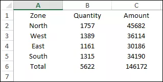
Applying formats with auto-format option is super simple. Let’s say you want to format below data table.
- Select any of the cells from your data.

- Go to the quick access toolbar and click on the auto-format button.
- Now, you have a window, where you have different data formats.
- Select one of them and click OK.


- Once you click OK, it will instantly apply your chosen format to the data.

How To Modify a Format in Auto Format
As I mentioned above, all the formats in the auto format are a combination of 6 different components. And you can also add or remove these components from each format before applying them.
Let’s say, you want to add formatting on the below data table but without changing its font style and column width. You need to apply formatting using the below steps.
- Select your data and click on auto-format button.
- Select a format to apply and click on the “Options” button.
- From options, un-tick “Font” and “Width/Height”.

- And, click OK.

Now, both of the components are not there in your formatting.
Removing Formatting
Well, to remove formatting from data the best way is to use a shortcut key Alt + H + E + F. But you can also use the auto format option to remove formatting from your data.
- Select your entire data and open auto format.
- Go to last in the format list where you have a “None” format.
